LoL: Using "Personality Quizzes" & Nearest Neighbors for Recommendations

This is the final in a 3-part series on recommendation methods, however I would consider this actually to be by far the most introductory of any article I’ve written and therefore would recommend starting here. For the experienced of you, I hope there is still value to be had — but you may want to skip a few introductory sections. I’ll make it clear in the article where these points are.

Previously, I’ve written about two recommendation methods:

“User-user collaborative filtering”: similar users like similar products.

“Content Based Model”: if a user likes a product, they’ll like similar products.

Today, we look at the iconic method: a Personality Quiz. Finding products most similar to the user based on their responses to a questionnaire. This is by far the least popular in “real-life”, as it adds too much friction and is relatively unreliable. However, it’s simple and provides a great introduction to the topic of recommendation engines whilst allowing more time to go through core concepts in detail. Also, they’re fun.

The Data Science technique used is called “Nearest Neighbors” and many people in the field would ostracize me for calling it Artificial Intelligence. Regardless, it forms the backbone of many applications that come later and therefore understanding it clearly should never be underappreciated.

As per most of my articles, I use the online game League of Legends (LoL) to apply the techniques. You don’t need to understand the game to understand the article, but here is an introduction to the game if you’d like to know more.

An Introduction to N-Dimensional Spaces

At some point in this article you will see “21-dimensional space”. This is where I lose some people. For non-mathematicians there can sometimes be the assumption that those people referring to any dimension past the 4th may in fact be communicating with the Gods, seeing into the future or are part lizard-alien. If you are nodding in agreement at this point, best to read this section in full. If you are quite familiar with what is meant by an N-dimensional space, please do skip ahead to An Introduction to Nearest Neighbors.

Let’s start simple. If I was studying a group of people, I may start by measuring all their weights. I have created a 1-dimensional space called “weight in KGs”. One person can only be heavier or lighter than the next. There is only one direction of travel. It is visualised by a simple straight line. Further left we go the lighter they are, the further right we go, the heavier they are.

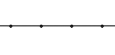
A 1-dimensional space, doesn’t get more simple than this! Image by Author.

Now we move to the 2-dimensional space by adding in their heights. We can plot every person in that space by going along to the weight, and up to their height. All very easy to visualise.

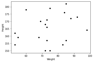
A 2D space of Height and Weight. Image by Author.

Things become a little more spicy at 3-dimensions when we include their annual salary. Picture a cube and imagine yourself at the closest, bottom left corner. You go along the width to their weight, up to the their height and then deeper into the cube depending on their salary. You could even jump inside that box with a ruler and measure the distance between two people to see how similar they are.

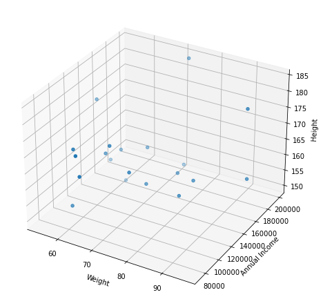
A 3D space, where the opacity of the points indicates the annual income. Image by Author.

However, what happens when I add shoe-size? We now have 4-dimensions. We are no longer able to mentally picture what this would look like — however nothing has changed! Those dots still appear in a space, it’s just that the space can’t be visually shown in our very boring 3D world. We can even still measure the distance between two points, it’s just we have to put the ruler away and do it mathematically.

This holds true whether we have 4-dimensions, 5-dimensions or 4,500-dimensions. It doesn’t matter! We can’t visualise anything past 3, but all the same principals and techniques can be applied (mathematically) in the same way no matter what size dimension we reach.

An Introduction to Nearest Neighbors

Whether you skipped here or read the above, I hope we’re all on the same page when I say “N-dimensional space”. This means we can move onto the actual technique itself.

Nearest Neighbors (NN) is exactly what it says on the tin. For any point in a space, find the N-number of nearest neighbors. Literally, you just pick a point and find the N-closest points to that one. “N” can be any number, however the standard Python implementation (sklearn) defaults to 5.

Hopefully, the visualisation below makes this crystal clear. Blue is the example point, Reds are the 5 nearest neighbors:

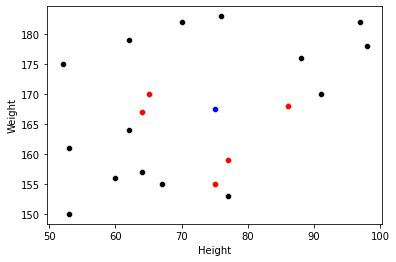
Visual explanation of Nearest Neighbors in a 2D space. Image by Author.

One thing to be clear on is what we mean when we say “nearest”. In the 2D space above we could just press a ruler to our screen, however what happens in the unimaginable 4-dimensional space and beyond? Well, we use the mathematical equivalent to a ruler: Euclidean distance.

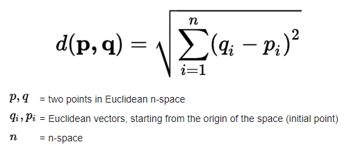
Euclidean Distance Equation. Source: Wikipedia.

Once again, the word “vector” is another trigger for many people. So let’s be explicit by what we mean (if you know all this, onto Applying Nearest Neighbors with you!).

Back to our population example. Let’s say we had the weight and height of two individuals.

Person 1: 70kg, 170cm

Person 2: 90kg, 185cm.

The weights are vectors (70, 90) and the heights are vectors (170, 185). As per the formula above, if we wanted to find the Euclidean distance between them we do the sum of the squared difference between each point. Like so:

Weight Squared Difference: (Person 1 Weight — Person 2 Weight) = (90–70)² = 20² = 400

Height Squared Difference: (Person 1 Height — Person 2 Height) =(185–170)² = 15² = 225

Square Root of (Weight Squared Difference + Height Squared Difference)) = Square Root(400 + 225) = Square Root(625) = 25.

The Euclidean Distance between individual one (70kg, 170cm) and individual two (90kg, 185cm) is 25.

If we instead were working with 4 dimensions (weight, height, income & shoe size) the values could be:

Person 1: 70kg, 170cm, $70,000, 10 Shoe Size

Person 2: 90Kg, 185cm, $95,000, 12 Shoe Size

The calculation is identical, except rather than just summing the squared difference between Heights and Weights, we also include Annual Salary and Shoe Size. Try working out the Euclidean Distance yourself. Answer is at the bottom of the article*.

Applying Nearest Neighbors to Personality Quizzes

But how does this all apply to recommending a League of Legends Champion (playable character) based on a personality quiz?

Here’s how it’s done:

Create a multi-dimensional space with features that help describe each Champion in the game (there’s currently 152 Champions to choose from).

Fit the NN algorithm to this space.

Create a survey that tries to place the person in that space.

Use the NN algorithm to determine the closest Champions to the survey representation of the person.

*Note: don’t worry if this doesn't make sense yet, we’re about to cover it in detail.*

Step 1. is by far the most cumbersome and time consuming. We build a script that fetches games from the Riot API and from these we extract the Champion played and in which lane. We also grab some features that we think will help describe the Champion, like how many kills they got, how much damage they did to objectives, how much damage they’ve blocked, etc…

I have this information for c. 8 million games, but that’s because I had it to hand from other projects. If you want to try this yourself, I wouldn’t suggest going that high.

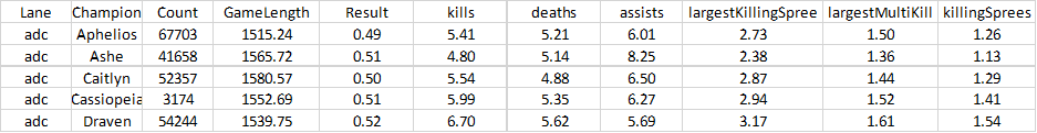
Here’s an example of what the table looks like, each row representing a Champions performance in one game:

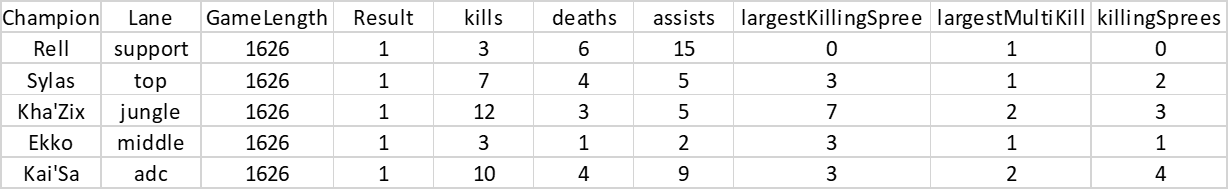
A table showing the Champions performance from one individual game. Image by Author.

We can then use a group-by on the dataframe to get the average values for each lane/Champion combination across all games. Here’s what that looks like:

# An aggregation dictionary allows you to do the mean for some values, and a sum for others.
# In our case we want to the average of all the columns, but count the number of games per champion

agg_dict = {'LaneType': 'count'}

for col in df.columns[4:]:
  agg_dict[col] = 'mean'

avg_champ_df = df.groupby(['Lane', 'Champion']).agg(agg_dict).reset_index()

A table showing a Champions average performance across many games. Image by Author.

Finally, I get rid of Lane/Champion combinations where there’s been less than 5,000 games. This removes really off-meta picks (<0.25% pick rate) and ensures there’s sufficient data for the averages to converge around their true mean (Central Limit Theorem).

We then split the dataframe into 5 by filtering by lane. You don’t need to do this, but I felt it was a cleaner process and I liked the idea of making individual recommendations per lane.

avg_champ_df = avg_champ_df[avg_champ_df['Count'] >= 5000]
top_champ_df = avg_champ_df[avg_champ_df['Lane'] == 'top']

I also created some additional features from the raw data that I thought would be interesting. For instance, I had the number of times a Champion killed someone without assistance (solo kills) and I also had their total number of kills. I created a new feature which was the percentage of their total kills which were solo (percentage of kills solo = solo kills / total kills).

The next step was to convert the dataframe into a matrix, where each row represents a Champion with 21 various statistics about their in-game performance on average across many samples.

We then normalize the data and fit the Nearest Neighbors algorithm to the matrix, with the default N = 5.

def normalization(row):
x_min, x_max = np.max(row), np.min(row)
return [(x - x_min) / (x_max - x_min) for x in row]

list_of_stats = [normalization(list(top_champ_df[x])) for x in stats]
# Initially it starts column-wise, (i.e. each list contains 1 stat across all champs)
XT = np.array(list_of_stats)
# So we transpose it to row-wise (i.e. each list contains all stats for 1 champ)
X = np.transpose(XT)

knn = NearestNeighbors(n_neighbors=5)
knn.fit(X)

A Side Note on Normalization

Again, this article really is intended for a reader of any level — so I don’t want to just write “we normalize the data” and move on without explaining and justifying myself. So, if you are comfortable with how/why we do this, skip this section. If not, here’s a quick explanation:

The Nearest Neighbors method we are using is entirely reliant on the Euclidean distance between two points. The problem we have is that each feature is on a different scale. For example, let’s take a Champion who on average deals 50,000 hits of damage and earns 10,000 gold per game.

We then want to measure the Euclidean distance between that Champion and one that does 50,000 hits of damage, but only gets 8,000 gold. Take a second to think about it…

…the answer is 2,000. Because the first number (damage: 50,000) isn’t changing, all the distance comes from the “gold” feature, where the difference is:

10,000 – 8,000 = 2,000.

Then we sum the two squared differences:

2,000² + 0² = 2,000²

Finally, take the square-root:

square-root(2,000²) = 2,000

So, for a 20% reduction in kills, the Euclidean distance is 2,000.

Now, imagine a Champion that instead only deals 40,000 hits of damage but still gets 5 kills. For a 20% reduction in damage, the Euclidean distance is now 10,000! This means the Nearest Neighbors algorithm will be 5x more reliant on the damage stat, than the kill stat. Hopefully this makes that clear:

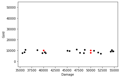
Observations with X: Damage, Y: Gold. Illustrating how the distance is far more reliant on Damage than Gold. Image by Author.

So, how do we fix it? We normalize the data. Or in other words, we make sure all statistics are in the same range between 0 and 1. To do this, we use the following:

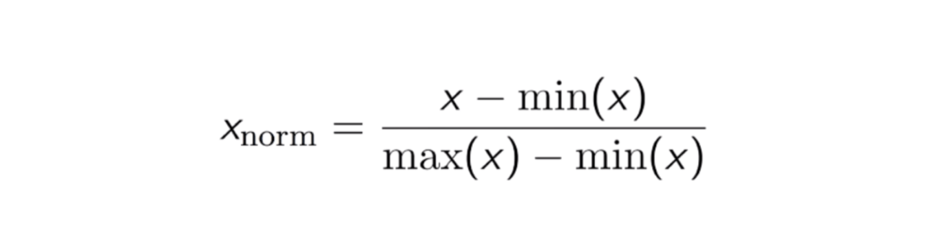
If the average Kills per game for 5 Champions were: [3, 1, 5, 6, 11].

min(x) = 1, max(x) = 11

Starting from the beginning of the list with x=3:

(x — min(x))/(max(x)-min(x))=(3 –1)/(11–1) = 2 / 10 = 0.2

If we do it to all the numbers in the list, [3, 1, 5, 6, 10]=>[0.2, 0, 0.4, 0.5, 1]

The Kills are now bound between 0 and 1. We do the same for Damage Dealt. Now changes in Kills are equally as powerful as changes in Damage.

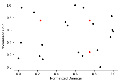
The same graph as above except both statistics are normalized. Now changes in Damage and Gold are equally powerful. Image by Author.

Converting Questionnaires into Data

Before we start, I’ll level with you. This part is as much art as science. Actually, it’s mostly art. Move forward with a large pinch of salt.

So, we have this 21-dimensional space (I told you it was coming). Each point represents a Champion and their position is dependent on a combination of these 21 statistics. Our next objective is to create a questionnaire which allows us to place the user into this space.

To do this, we need to find out a rough approximation for each of the 21 statistics based on the “personality” of the survey taker. In other words, for each statistic, there needs to be a corresponding question and a way of translating their answer into a usable number.

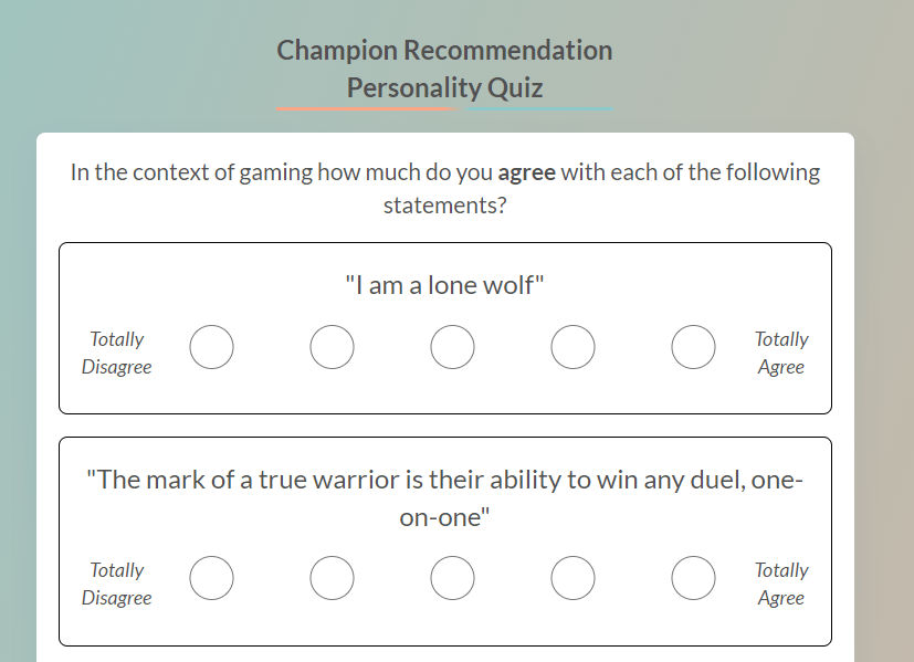
For this, I opted for the “How much do you agree with the following statement” style of questions. The reason it works well is because they respond on a scale, which I set as:

Total Disagree, Disagree, Neutral, Agree, Totally Agree

I can then convert these statements into percentiles, which then converts into data. An example should help make this clearer:

The first statistic in our dataset is: percentage of a Champion kills which were done without assistance. I (artfully) translated that to the following statement:

“I am a lone wolf”

Why? Champions with a high % are people who get most of their kills when acting alone. Those with a low % rely on their team mates to help secure kills. Hence, lone wolf. This is the art of science part.

So, those who respond to this statement with “Totally Agree” are assumed to have the top 20% percentile of the statistic whilst those responding “Totally Disagree” are in the bottom 20%. Those who say Neutral are somewhere between 40–60%. Given we have this statistic for all Champions, we just calculate a rough estimate of what their value would be.

To help clarify this, let’s imagine I only had 10 Champions and I was looking at the number of Kills they average per game:

Kills per Game = [1, 1, 2, 3, 3, 3, 4, 5, 7, 8]

If someone said “Totally Disagree” to a statement relating to Kills per Game (such as “I like to get lots of kills”), that puts them in the bottom 20% of this statistic. So, the bottom 20% of the 10 Champions is the bottom 2. For this person, we’d give them Kills per Game of 1. Why? The lowest 2 values in the list above are 1 & 1.

If someone else said “Totally Agree”, they’d be in the top 20%. So either 7 or 8 kills per game.

How about “Agree”? It’s somewhere between 60–80%, so 4 or 5. You get the picture.

We then continue creating questions out of the 21 statistics available, each time converting their answer to an actual value. A full list of the questions and their related statistics can be found here:

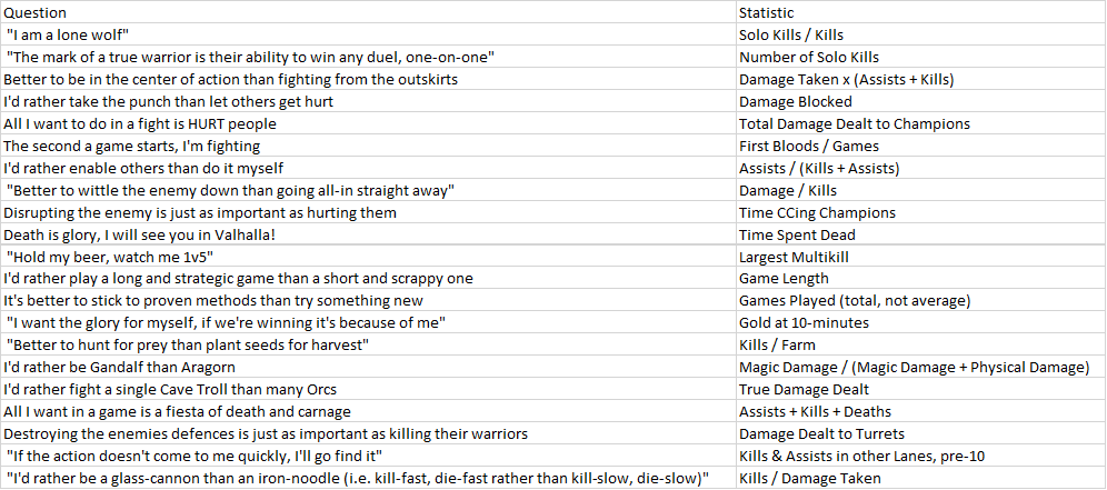
Now, when someone completes the “Personality Quiz”, we convert each answer to a statistic, normalize the values (using the same min/max values we used on the original dataset) and boom — we have converted their personality to a position in our 21-dimensional space!

The final step is to use the NN algorithm we fit earlier to determine which of the original Champions are closest to this persons response and provide them the top 5 as recommendations!

A Final Note

Some of you may be asking “but in the example above you said that Totally Agree could EITHER be 7 or 8, how do you choose?”. The answer is, I don’t. I used a random number generator to pick a value in the range. That means each time you answer the quiz you get slightly different answers, given that your own point in space randomly moves within a 20% range and so different Champions become closer/further away. One alterative method would be to stick with a static answer (i.e. the mid-point of 7 or 8 = 7.5), however that means you get less Champion diversity in the responses. Another option would be to say “On a scale of 1 to 1,000 how much do you agree with the statement”, but that didn’t feel very user friendly. There’s no right answer here.

If you’d like to try the finished product for yourself, you’ll find it here. I’d love to hear whether you agree with the results or not!

This article is considerably more detailed than I usually write, I spent a lot of time labouring over the explanations for more fundamental concepts like dimensional space and normalization. This is because I wanted somewhere to refer someone completely new into the field (as I’m meeting a lot of them at the moment with my work). However, I hope there’s still a few veterans that found just enough interesting material to make it worth the read.